Setting Up Your Python Environment

Petroleum engineering runs on calculation. Every well drilled, every reservoir modeled, every production forecast issued depends on numbers (pressures, flow rates, fluid properties, rock characteristics) computed correctly and applied with judgment. For decades, engineers ran these calculations by hand, then in spreadsheets, then in expensive commercial software. Python changes that. It costs nothing, runs on any machine, and scales from a single pressure calculation to a reservoir simulation with millions of grid cells.

This chapter does two things. First, it gives you a working Python environment on your own machine, with every library you will need for the rest of this book. Second, it introduces the petroleum industry itself: what it is, how it works, and why computation sits at the center of it. By the end, you will write your first engineering calculation: the hydrostatic pressure equation, the formula that keeps wells from blowing out.

Petroleum engineering is the discipline of finding hydrocarbons trapped deep underground, bringing them to the surface, and managing the reservoir so that it produces as much as economically possible over its lifetime. It is one of the most capital-intensive industries on earth. A single offshore well can cost over a hundred million dollars. The decisions petroleum engineers make (where to drill, how deep, what fluids to pump, when to shut a well in) are backed by physics, geology, chemistry, and increasingly, computation.

If you are new to this field, what follows is the foundation you need before any code will make sense. If you already work in the industry, treat this as a refresher and pay attention to where Python fits into each phase.

Crude oil is not sitting in an underground lake. That is the most common misconception, and it matters because it shapes how you think about every calculation in this book.

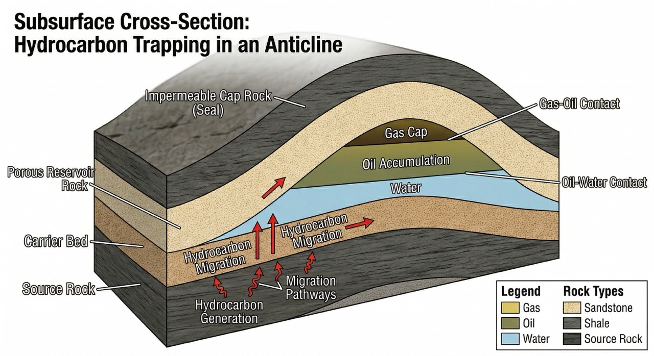
Hundreds of millions of years ago, tiny marine organisms (plankton, algae) died and settled on the ocean floor. Layer after layer of sediment buried them. The organic-rich rock that locked away their remains is the source rock. As that rock subsided to greater depth, heat and pressure transformed the buried organic matter into a waxy intermediate called kerogen, and then, once temperatures crossed roughly 60 °C, typically a burial depth of two to three kilometres, into liquid hydrocarbons. Geologists call this the oil window. Push a basin deeper, past about 120 °C, and the same source rock starts cracking its hydrocarbons into natural gas: the gas window. Whether a basin produces oil, gas, or both is largely a question of how deep its source rock buried, how hot it got, and for how long.

The hydrocarbons that formed in the source rock did not stay there. Buoyancy drove them upward through whatever porous rock would let them through, until they hit an impermeable barrier (a cap rock, or seal) and stopped. The porous rock formation where hydrocarbons accumulate beneath that seal is the reservoir. Three things have to coexist for an economic accumulation: a source rock that generated the hydrocarbons, a reservoir rock with enough porosity and permeability to hold and release them, and a seal that trapped them. Miss any one of the three and there is nothing to drill.

A reservoir is, in effect, a kitchen sponge soaked with oil, buried two miles underground and sealed under solid shale. You cannot see it directly. You infer its properties from indirect measurements, and then you calculate.

Every oil and gas project follows a broad lifecycle, and computation runs through every stage:

1. Exploration: Geologists and geophysicists hunt for promising structures with seismic surveys and surface geology, asking one question: is there a trap down there that might hold hydrocarbons? Seismic processing is among the most computationally demanding tasks in any industry.
2. Appraisal and Drilling: Wells are drilled to confirm the resource. Each is a multi-million-dollar bet, and the calculations governing mud weight, casing design, and wellbore stability decide whether that bet pays off.
3. Production: Hydrocarbons flow to surface while engineers monitor pressures, rates, and fluid compositions, optimize artificial lift as pressure declines, and forecast ultimate recovery. Every one of those tasks is data, models, and code.
4. Abandonment: Every well eventually stops producing economically and is plugged, its equipment removed and the site restored, with its own set of calculations and regulatory requirements.

The thread through all four phases: you are deciding about rock you cannot see, thousands of feet down, from indirect measurements (pressures, flow tests, well logs, seismic images). Python is the tool that turns those measurements into engineering decisions.

Python is a general-purpose language; the petroleum work in this book runs on a specific stack of scientific libraries. Installing that stack cleanly now, the same libraries, the same way, as everyone else, is what lets a calculation you write in chapter 8 run unchanged on a colleague's laptop or a field server two years later. Rather than installing each library separately, we use Anaconda, a free Python distribution that bundles everything in a single download.

Anaconda bundles the libraries this book relies on:

• NumPy: numerical arrays and linear algebra; the backbone of every calculation here.
• Pandas: tabular data: production records, well headers, fluid-property tables.
• Matplotlib: plots: decline curves, pressure-depth profiles, well log displays.
• SciPy: curve fitting, optimization, and numerical integration.
• Jupyter: interactive notebooks that mix code, results, and notes in one file.

1. Go to anaconda.com/download and download the installer for your operating system (Windows, macOS, or Linux).
2. Run the installer and accept the defaults. On Windows, choose "Just Me" for the installation type and check "Add Anaconda to PATH" when prompted.
3. Open a terminal (on Windows, open Anaconda Prompt from the Start Menu) and verify the installation:

You should see Python 3.11.x or Python 3.12.x. Any version 3.9 or above works for this book.

1. Confirm the core libraries are available:

If that runs without errors, your installation is complete. The following code block verifies it from inside Python and reports the version numbers:

If you see an ImportError, Anaconda was likely not installed correctly. Revisit the steps above, or check that you are running Python from the Anaconda environment rather than a system Python.

You will use two tools throughout this book, and the choice between them is practical, not cosmetic. A one-off water-cut check belongs in a notebook you step through cell by cell; a forecast tool that has to run every night against the production database belongs in a versioned script. Pick the wrong one and you either lose your exploratory history or end up babysitting a notebook nobody can schedule.

A Jupyter Notebook is an interactive document made up of cells. Each cell contains either Python code or formatted text. When you run a code cell (Shift + Enter), the output appears directly below it. This makes notebooks ideal for exploratory analysis: you build a calculation one step at a time, inspect the results, adjust, and continue.

In petroleum engineering, notebooks are where you will analyze well logs and production data, build and test decline curve models, create pressure-depth plots and other visualizations, and document your assumptions alongside your calculations so that a colleague (or your future self) can follow the reasoning.

To launch Jupyter, open a terminal and type:

A browser window opens with a file navigator. Click New → Python 3 to create a notebook, then run cells with Shift + Enter. The rest of the shortcuts (Esc B to add a cell, Esc M to switch a cell to Markdown) you pick up by using them.

When your work grows beyond a single notebook, when you write reusable functions, build multi-file projects, or create scripts that run on a schedule, you need a code editor. Visual Studio Code (VS Code) is free, fast, and widely used in both software engineering and data science.

To set it up:

1. Download VS Code from code.visualstudio.com.
2. Install the Python extension by Microsoft (search in the Extensions panel).
3. Install the Jupyter extension to run notebooks directly inside VS Code.

Use Jupyter when you are exploring data and testing ideas. Use VS Code when you are building tools meant to last. This book uses both.

Before we get to engineering formulas, let's confirm that your environment works by building something practical: a well information card, the kind of summary that appears at the top of every well report in the industry.

Every variable is named using petroleum terminology: well_name, target_depth_ft, spud_date. This is a deliberate practice. When you read mud_weight_ppg later in this chapter, you will know immediately that it holds a mud weight measured in pounds per gallon. Code written this way is readable by engineers, not just programmers.

This is your first real engineering calculation, and it is worth understanding why it exists before you see the formula.

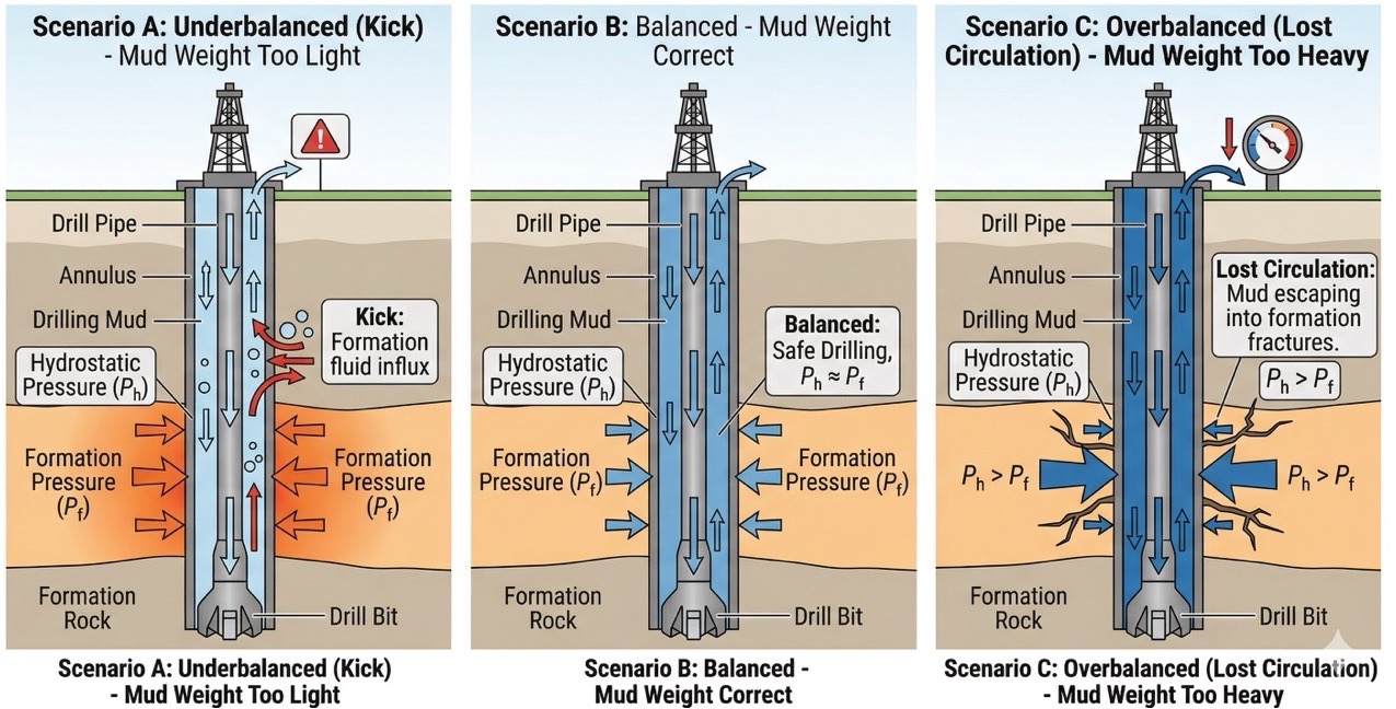
When you drill a well, you continuously pump a fluid (called drilling mud) down through the inside of the drill pipe, out through nozzles in the bit, and back up the space between the pipe and the rock (the annulus). This circulating mud serves several purposes: it cools the bit, carries rock cuttings to the surface, and stabilizes the wellbore walls. But its most critical function is pressure control.

Deep underground, rock formations contain fluids (oil, gas, water) under enormous natural pressure. The column of drilling mud in the wellbore must exert enough pressure to hold those formation fluids in place.

If the mud is too light, it cannot counterbalance the formation pressure. Formation fluids enter the wellbore: a kick. If a kick is not controlled, it escalates into a blowout: an uncontrolled release of hydrocarbons to surface. Blowouts are among the most dangerous events in the industry. People die. Equipment is destroyed. Environmental damage can last decades. The 2010 Macondo blowout in the Gulf of Mexico killed eleven workers and triggered the largest marine oil spill in U.S. history, a chain of failures that began, in part, with mud weight and pressure decisions made in the days leading up to the event.

If the mud is too heavy, it exerts more pressure than the rock can withstand. The formation fractures, and mud pours into the cracks: lost circulation. You lose expensive fluid, you may damage the reservoir you are trying to produce from, and in severe cases, you lose the well entirely.

The difference between "too light" and "too heavy" can be less than one pound per gallon. Getting it right is not optional. It starts with one equation.

The pressure at the bottom of a column of fluid depends on two things: the density of the fluid and the height of the column. In oilfield units:

where:

• $P$ = hydrostatic pressure in psi (pounds per square inch)
• $MW$ = mud weight in ppg (pounds per gallon)
• $TVD$ = true vertical depth in feet
• $0.052$ = a unit conversion constant that reconciles ppg, feet, and psi

This formula is one of the first things a drilling engineer learns, and one of the last things they stop using. Let's implement it.

The if/else block at the end is your first piece of engineering logic in Python: it checks whether the well is under control and reports the result, the same check a drilling engineer makes before every operation.

In practice, you rarely calculate hydrostatic pressure at a single depth. A well has multiple casing strings set at different depths, and the drilling team needs to know the pressure at each one. Here is how you build that table in Python instead of a spreadsheet.

If the mud weight changes tomorrow, you change one variable. If the well plan adds a casing string, you add one dictionary entry. The code handles the rest. Python replaces spreadsheets for engineering work not because it is fancier, but because it is faster to maintain and harder to break.

A printed table gives the numbers; a plot gives the shape. The pressure-depth profile is the most-read chart in any drilling office, so let's draw the one we just computed.

The line is straight because mud weight is constant; the slope is the pressure gradient (0.052 × MW = 0.582 psi/ft). When mud weight changes between sections, the line breaks. Reading those breakpoints is part of what a drilling engineer does every day.

• The petroleum industry is the business of finding, extracting, and managing hydrocarbons trapped in rock formations underground. Engineers make decisions about resources they cannot see directly, relying on data and calculation.
• Crude oil forms from ancient organic matter subjected to heat and pressure over geological time. It accumulates in porous rock (the reservoir) sealed by impermeable cap rock.
• The petroleum lifecycle spans exploration, drilling, production, and abandonment. Computation plays a role in every phase.
• Anaconda bundles Python with NumPy, Pandas, Matplotlib, SciPy, and Jupyter: the core tools for petroleum engineering computation.
• Jupyter Notebooks are suited to interactive analysis and documentation. VS Code is suited to building reusable tools and multi-file projects.
• Hydrostatic pressure ($P = 0.052 \times MW \times TVD$) is one of the most fundamental calculations in drilling engineering. The mud weight must be heavy enough to prevent a kick but light enough to avoid fracturing the formation. Getting it wrong has serious consequences.
• Variable naming matters. Names like mud_weight_ppg, tvd_ft, and formation_pressure_psi carry their units, so the calculation documents itself.